Bound a prediction from an uncertain observation
A recorded execution cost may be known only within a range. Instead of choosing a fitted parameter, keep every parameter consistent with that observation and carry the resulting uncertainty into a planned execution. This small example explores solution families; its linear impact law is illustrative.
Define an execution’s mathematics once:
class Execution(Modello):
    """A deliberately small model: price impact is linear in trade quantity."""

    quantity = InstanceDummy("quantity", positive=True)
    reference = InstanceDummy("reference", positive=True)
    impact = InstanceDummy("impact", nonnegative=True)
    fee = InstanceDummy("fee", nonnegative=True)
    price = reference + impact * quantity
    cost = quantity * price + fee
Join two executions through the same impact coefficient:
class ImpactStudy(Modello):
    """Recorded and planned executions share their impact coefficient."""

    recorded = component(Execution)
    planned = component(Execution)
    impact = recorded.impact
    impact = planned.impact
Fix the quantities, reference prices, and fees. Impact remains unknown:
    @classmethod
    def prepare(cls) -> ModelProblem[ImpactStudy]:
        """Fix the observed trade terms and the proposed trade size."""
        return inspect_model(
            cls,
            "impact study",
            recorded=Execution("recorded", quantity=2, reference=99, fee=1),
            planned=Execution("planned", quantity=10, reference=100, fee=1),
        )
>>> from examples.solution_families import ImpactStudy
>>> problem = ImpactStudy.prepare()
>>> study = problem.symbols
>>> family = problem.solutions(study.impact)
Keep impact as the exploration coordinate. Constrain the recorded cost to its observed interval, then ask what that means for the planned trade:
>>> calibrated = family.where(study.recorded.cost >= 200, study.recorded.cost <= 202)
>>> calibrated.values(study.impact)
Interval(1/4, 3/4)
The joining model carries the calibration into the prediction through one
shared quantity. ImpactStudy.calibrated() packages these preparation and
observation steps into a prediction that is ready to query:
>>> prediction = ImpactStudy.calibrated()
>>> prediction.values(prediction.symbols.planned.cost)
Interval(1026, 1076)
>>> prediction.expression(prediction.symbols.planned.cost) == 100 * prediction.symbols.impact + 1001
True
There is no statistical confidence level attached to this interval; it follows from the specified bounds and the model’s assumptions.
Select a particular impact to obtain a normal typed model:
>>> from sympy import Rational
>>> case = prediction.observe(impact=Rational(1, 2)).one()
>>> case.recorded.cost, case.planned.cost
(201, 1051)
>>> case.recorded.impact == case.planned.impact
True
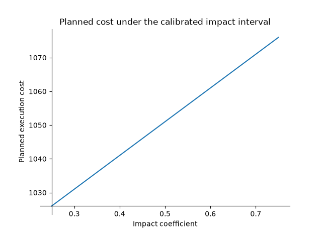
Plot the same expression over its admissible interval with
ImpactStudy.plot(prediction, Path("cost.png")). From a checkout, the
notebook dependency group supplies the optional Matplotlib backend:
$ uv run --group notebooks python -m examples.solution_families --plot cost.png
Running python -m examples.solution_families prints the intervals with only
the library’s existing SymPy dependency. The plot is a view of the bounded
family; numerical plotting does not establish additional guarantees.
Discover where a projectile can reach
A thrown ball gives familiar, nonlinear geometry from one physical model.
Assume uniform gravity and no air resistance. FreeFlight describes where
it would be at the same time without gravity: x, y are horizontal and
z is vertical. At a fixed speed, squared distance determines squared
travel time. Projectile subtracts the gravitational drop:
class FreeFlight(Modello):
    """Where the throw would be at the same time without gravity, in metres."""

    speed = InstanceDummy("speed", positive=True)
    x = InstanceDummy("x", real=True)
    y = InstanceDummy("y", real=True)
    z = InstanceDummy("z", real=True)
    time_squared = (x**2 + y**2 + z**2) / speed**2


class Projectile(Modello):
    """A throw from the origin under uniform gravity, without air resistance."""

    free = component(FreeFlight)
    gravity = InstanceDummy("gravity", positive=True)
    x = free.x
    y = free.y
    target_height = InstanceDummy("target_height", real=True)
    height = free.z - gravity * free.time_squared / 2
    clearance = height - target_height
Fix launch speed at 20 m/s and gravity at 10 m/s², leaving destinations unknown:
>>> from examples.projectile import FreeFlight, Projectile
>>> from sympy import Eq, FiniteSet, diff, factor
>>> problem = Projectile.prepare()
>>> flight = problem.symbols
>>> family = problem.solutions(flight.x, flight.y, flight.free.z, flight.target_height)
First solve backwards: which launch directions reach a target 16 metres away and 16 metres high? Both a lower and a higher throw satisfy the same model:
>>> hits = family.observe(x=16, y=0, target_height=16).where(Eq(flight.clearance, 0))
>>> hits.values(flight.free.z) == FiniteSet(32, 48)
True
>>> len(hits.cases())
2
To find the boundary of all reachable targets, expand the height expression before differentiating its vertical free-flight coordinate. Varying that coordinate changes launch direction and travel time while holding the horizontal destination fixed:
>>> height = family.expression(flight.height)
>>> stationary = diff(height, flight.free.z)
>>> envelope = family.where(Eq(stationary, 0))
SymPy derives the maximum reachable height at every horizontal location:
>>> ceiling = envelope.expression(flight.height)
>>> ceiling == 20 - flight.x**2 / 80 - flight.y**2 / 80
True
>>> factor(ceiling - height) == (flight.free.z - 40)**2 / 80
True
The nonnegative square proves this is a global maximum, rather than merely a
stationary point. This trajectory envelope bounds a family of throws; it
is not itself one ball’s trajectory. Projectile.envelope() packages these
same derivation steps, without introducing another height formula.
Take sections through a typed reference. With sideways displacement zero, the envelope is the parabola of safety:
>>> reference = envelope.observe(x=0, y=0, target_height=0).one()
>>> curve = envelope.section(flight.x, through=reference)
>>> curve.expression(flight.height) == 20 - flight.x**2 / 80
True
Instead, vary horizontal distance and target height. Keeping targets above ground and below the envelope selects the reachable area in that plane:
>>> plane = envelope.section(flight.x, flight.target_height, through=reference)
>>> area = plane.where(flight.target_height >= 0, flight.clearance >= 0)
Allow both horizontal coordinates to vary for the safety paraboloid. Allow target height to vary too, under the same constraints, for the reachable volume:
>>> surface = envelope.section(flight.x, flight.y, through=reference)
>>> volume = envelope.where(flight.target_height >= 0, flight.clearance >= 0)
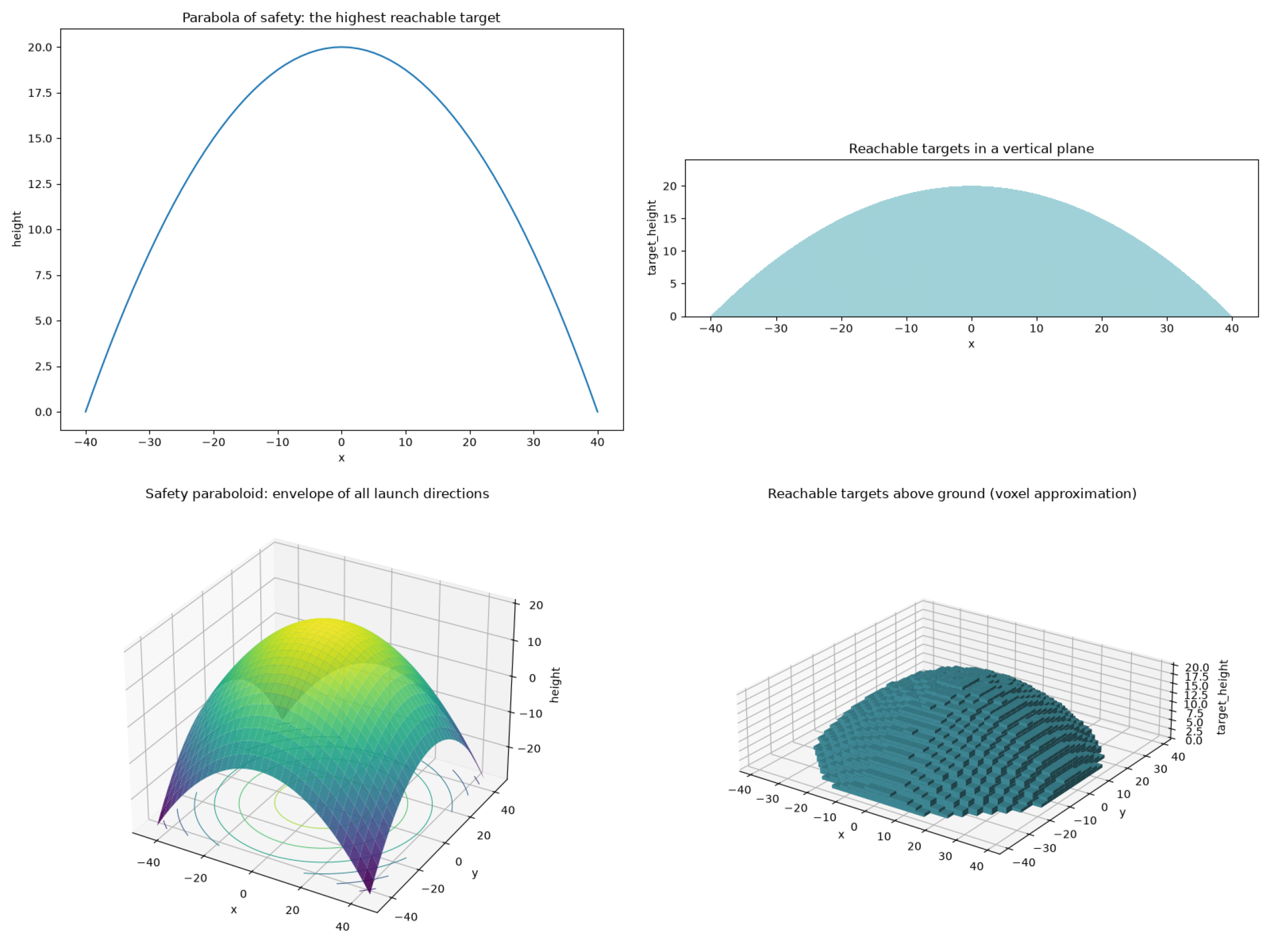
One motion model supplies a curve, area, surface, and volume. The volume uses occupied voxel centres; cells may cross the exact boundary. The surface also shows its continuation below ground.
A surface has two independent controls even though its scalar height response has a one-dimensional image. Include the coordinates when measuring its graph:
>>> from examples.solution_views import ModelView
>>> view = ModelView(surface.parameters, surface)
>>> view.control_dimension, view.image_dimension(flight.x, flight.y, flight.height)
(2, 2)
ModelViews.sections() lazily enumerates coordinate sections through the
reference. Export these four named views with optional notebook dependencies:
$ uv run --group notebooks python -m examples.solution_views --plot-dir views
Open views/index.html. ModelView.plot(...) draws polynomial responses;
plot_region(...) draws planar implicit sets or approximates spatial
inequality regions. Both take typed lower and upper models as windows.
Numerical pictures do not establish dimensions or exact boundaries.
Dimension reporting covers real interval boxes and finite point sets;
polynomial image dimension uses exact rational-function Jacobian rank
(Geiger et al., Lemma 9 and Theorem 10).
Coupled domains remain None even when their geometry looks clear. These
constraints still define exact sets when SymPy retains a ConditionSet.
To explore a supplied input, prepare a new problem leaving it unknown;
observations add constraints rather than unpinning existing inputs.
The equations follow OpenStax’s projectile motion model. The gravity-free coordinates and envelope construction follow Mark Levi’s Parabola of Safety and the Jacobian.